![]()
Boston Housing Dataset
The Boston data frame has 506 rows and 14 columns.This dataframe contains the following columns:
CRIM = per capita crime rate by town.
ZN = proportion of residential land zoned for lots over 25,000 sq.ft.
INDUS = proportion of non-retail business acres per town.
CHAS = Charles River dummy variable (= 1 if tract bounds river; 0 otherwise).
NOX = nitrogen oxides concentration (parts per 10 million).
RM = average number of rooms per dwelling.
AGE = proportion of owner-occupied units built prior to 1940.
DIS = weighted mean of distances to five Boston employment centres.
RAD = index of accessibility to radial highways.
TAX = full-value property-tax rate per $10,000.
PTRATIO = pupil-teacher ratio by town.
BLACK = 1000(Bk - 0.63)^2 where Bk is the proportion of blacks by town.
LSTAT = lower status of the population (percent).
price = median value of owner-occupied homes in $1000s
** Price is the TARGET variable **
import numpy as np
import pandas as pd
import seaborn as sns
import matplotlib.pyplot as plt
%matplotlib inline
from sklearn.datasets import load_boston

from sklearn.model_selection import train_test_split
from sklearn.linear_model import LinearRegression
from sklearn.metrics import mean_absolute_error, mean_squared_error
boston = load_boston()
type(boston)
sklearn.utils.Bunch
boston.feature_names
array(['CRIM', 'ZN', 'INDUS', 'CHAS', 'NOX', 'RM', 'AGE', 'DIS', 'RAD',
       'TAX', 'PTRATIO', 'B', 'LSTAT'], dtype='<U7')
data = boston.data
type(data)
numpy.ndarray
data.shape
(506, 13)
data = pd.DataFrame(data = data, columns= boston.feature_names)
data.head()
| CRIM | ZN | INDUS | CHAS | NOX | RM | AGE | DIS | RAD | TAX | PTRATIO | B | LSTAT | |
|---|---|---|---|---|---|---|---|---|---|---|---|---|---|
| 0 | 0.00632 | 18.0 | 2.31 | 0.0 | 0.538 | 6.575 | 65.2 | 4.0900 | 1.0 | 296.0 | 15.3 | 396.90 | 4.98 |
| 1 | 0.02731 | 0.0 | 7.07 | 0.0 | 0.469 | 6.421 | 78.9 | 4.9671 | 2.0 | 242.0 | 17.8 | 396.90 | 9.14 |
| 2 | 0.02729 | 0.0 | 7.07 | 0.0 | 0.469 | 7.185 | 61.1 | 4.9671 | 2.0 | 242.0 | 17.8 | 392.83 | 4.03 |
| 3 | 0.03237 | 0.0 | 2.18 | 0.0 | 0.458 | 6.998 | 45.8 | 6.0622 | 3.0 | 222.0 | 18.7 | 394.63 | 2.94 |
| 4 | 0.06905 | 0.0 | 2.18 | 0.0 | 0.458 | 7.147 | 54.2 | 6.0622 | 3.0 | 222.0 | 18.7 | 396.90 | 5.33 |
boston.target
array([24. , 21.6, 34.7, 33.4, 36.2, 28.7, 22.9, 27.1, 16.5, 18.9, 15. ,
       18.9, 21.7, 20.4, 18.2, 19.9, 23.1, 17.5, 20.2, 18.2, 13.6, 19.6,
       15.2, 14.5, 15.6, 13.9, 16.6, 14.8, 18.4, 21. , 12.7, 14.5, 13.2,
       13.1, 13.5, 18.9, 20. , 21. , 24.7, 30.8, 34.9, 26.6, 25.3, 24.7,
       21.2, 19.3, 20. , 16.6, 14.4, 19.4, 19.7, 20.5, 25. , 23.4, 18.9,
       35.4, 24.7, 31.6, 23.3, 19.6, 18.7, 16. , 22.2, 25. , 33. , 23.5,
       19.4, 22. , 17.4, 20.9, 24.2, 21.7, 22.8, 23.4, 24.1, 21.4, 20. ,
       20.8, 21.2, 20.3, 28. , 23.9, 24.8, 22.9, 23.9, 26.6, 22.5, 22.2,
       23.6, 28.7, 22.6, 22. , 22.9, 25. , 20.6, 28.4, 21.4, 38.7, 43.8,
       33.2, 27.5, 26.5, 18.6, 19.3, 20.1, 19.5, 19.5, 20.4, 19.8, 19.4,
       21.7, 22.8, 18.8, 18.7, 18.5, 18.3, 21.2, 19.2, 20.4, 19.3, 22. ,
       20.3, 20.5, 17.3, 18.8, 21.4, 15.7, 16.2, 18. , 14.3, 19.2, 19.6,
       23. , 18.4, 15.6, 18.1, 17.4, 17.1, 13.3, 17.8, 14. , 14.4, 13.4,
       15.6, 11.8, 13.8, 15.6, 14.6, 17.8, 15.4, 21.5, 19.6, 15.3, 19.4,
       17. , 15.6, 13.1, 41.3, 24.3, 23.3, 27. , 50. , 50. , 50. , 22.7,
       25. , 50. , 23.8, 23.8, 22.3, 17.4, 19.1, 23.1, 23.6, 22.6, 29.4,
       23.2, 24.6, 29.9, 37.2, 39.8, 36.2, 37.9, 32.5, 26.4, 29.6, 50. ,
       32. , 29.8, 34.9, 37. , 30.5, 36.4, 31.1, 29.1, 50. , 33.3, 30.3,
       34.6, 34.9, 32.9, 24.1, 42.3, 48.5, 50. , 22.6, 24.4, 22.5, 24.4,
       20. , 21.7, 19.3, 22.4, 28.1, 23.7, 25. , 23.3, 28.7, 21.5, 23. ,
       26.7, 21.7, 27.5, 30.1, 44.8, 50. , 37.6, 31.6, 46.7, 31.5, 24.3,
       31.7, 41.7, 48.3, 29. , 24. , 25.1, 31.5, 23.7, 23.3, 22. , 20.1,
       22.2, 23.7, 17.6, 18.5, 24.3, 20.5, 24.5, 26.2, 24.4, 24.8, 29.6,
       42.8, 21.9, 20.9, 44. , 50. , 36. , 30.1, 33.8, 43.1, 48.8, 31. ,
       36.5, 22.8, 30.7, 50. , 43.5, 20.7, 21.1, 25.2, 24.4, 35.2, 32.4,
       32. , 33.2, 33.1, 29.1, 35.1, 45.4, 35.4, 46. , 50. , 32.2, 22. ,
       20.1, 23.2, 22.3, 24.8, 28.5, 37.3, 27.9, 23.9, 21.7, 28.6, 27.1,
       20.3, 22.5, 29. , 24.8, 22. , 26.4, 33.1, 36.1, 28.4, 33.4, 28.2,
       22.8, 20.3, 16.1, 22.1, 19.4, 21.6, 23.8, 16.2, 17.8, 19.8, 23.1,
       21. , 23.8, 23.1, 20.4, 18.5, 25. , 24.6, 23. , 22.2, 19.3, 22.6,
       19.8, 17.1, 19.4, 22.2, 20.7, 21.1, 19.5, 18.5, 20.6, 19. , 18.7,
       32.7, 16.5, 23.9, 31.2, 17.5, 17.2, 23.1, 24.5, 26.6, 22.9, 24.1,
       18.6, 30.1, 18.2, 20.6, 17.8, 21.7, 22.7, 22.6, 25. , 19.9, 20.8,
       16.8, 21.9, 27.5, 21.9, 23.1, 50. , 50. , 50. , 50. , 50. , 13.8,
       13.8, 15. , 13.9, 13.3, 13.1, 10.2, 10.4, 10.9, 11.3, 12.3,  8.8,
        7.2, 10.5,  7.4, 10.2, 11.5, 15.1, 23.2,  9.7, 13.8, 12.7, 13.1,
       12.5,  8.5,  5. ,  6.3,  5.6,  7.2, 12.1,  8.3,  8.5,  5. , 11.9,
       27.9, 17.2, 27.5, 15. , 17.2, 17.9, 16.3,  7. ,  7.2,  7.5, 10.4,
        8.8,  8.4, 16.7, 14.2, 20.8, 13.4, 11.7,  8.3, 10.2, 10.9, 11. ,
        9.5, 14.5, 14.1, 16.1, 14.3, 11.7, 13.4,  9.6,  8.7,  8.4, 12.8,
       10.5, 17.1, 18.4, 15.4, 10.8, 11.8, 14.9, 12.6, 14.1, 13. , 13.4,
       15.2, 16.1, 17.8, 14.9, 14.1, 12.7, 13.5, 14.9, 20. , 16.4, 17.7,
       19.5, 20.2, 21.4, 19.9, 19. , 19.1, 19.1, 20.1, 19.9, 19.6, 23.2,
       29.8, 13.8, 13.3, 16.7, 12. , 14.6, 21.4, 23. , 23.7, 25. , 21.8,
       20.6, 21.2, 19.1, 20.6, 15.2,  7. ,  8.1, 13.6, 20.1, 21.8, 24.5,
       23.1, 19.7, 18.3, 21.2, 17.5, 16.8, 22.4, 20.6, 23.9, 22. , 11.9])
data['Price'] = boston.target
data.head()
| CRIM | ZN | INDUS | CHAS | NOX | RM | AGE | DIS | RAD | TAX | PTRATIO | B | LSTAT | Price | |
|---|---|---|---|---|---|---|---|---|---|---|---|---|---|---|
| 0 | 0.00632 | 18.0 | 2.31 | 0.0 | 0.538 | 6.575 | 65.2 | 4.0900 | 1.0 | 296.0 | 15.3 | 396.90 | 4.98 | 24.0 |
| 1 | 0.02731 | 0.0 | 7.07 | 0.0 | 0.469 | 6.421 | 78.9 | 4.9671 | 2.0 | 242.0 | 17.8 | 396.90 | 9.14 | 21.6 |
| 2 | 0.02729 | 0.0 | 7.07 | 0.0 | 0.469 | 7.185 | 61.1 | 4.9671 | 2.0 | 242.0 | 17.8 | 392.83 | 4.03 | 34.7 |
| 3 | 0.03237 | 0.0 | 2.18 | 0.0 | 0.458 | 6.998 | 45.8 | 6.0622 | 3.0 | 222.0 | 18.7 | 394.63 | 2.94 | 33.4 |
| 4 | 0.06905 | 0.0 | 2.18 | 0.0 | 0.458 | 7.147 | 54.2 | 6.0622 | 3.0 | 222.0 | 18.7 | 396.90 | 5.33 | 36.2 |
data.describe()
| CRIM | ZN | INDUS | CHAS | NOX | RM | AGE | DIS | RAD | TAX | PTRATIO | B | LSTAT | Price | |
|---|---|---|---|---|---|---|---|---|---|---|---|---|---|---|
| count | 506.000000 | 506.000000 | 506.000000 | 506.000000 | 506.000000 | 506.000000 | 506.000000 | 506.000000 | 506.000000 | 506.000000 | 506.000000 | 506.000000 | 506.000000 | 506.000000 |
| mean | 3.613524 | 11.363636 | 11.136779 | 0.069170 | 0.554695 | 6.284634 | 68.574901 | 3.795043 | 9.549407 | 408.237154 | 18.455534 | 356.674032 | 12.653063 | 22.532806 |
| std | 8.601545 | 23.322453 | 6.860353 | 0.253994 | 0.115878 | 0.702617 | 28.148861 | 2.105710 | 8.707259 | 168.537116 | 2.164946 | 91.294864 | 7.141062 | 9.197104 |
| min | 0.006320 | 0.000000 | 0.460000 | 0.000000 | 0.385000 | 3.561000 | 2.900000 | 1.129600 | 1.000000 | 187.000000 | 12.600000 | 0.320000 | 1.730000 | 5.000000 |
| 25% | 0.082045 | 0.000000 | 5.190000 | 0.000000 | 0.449000 | 5.885500 | 45.025000 | 2.100175 | 4.000000 | 279.000000 | 17.400000 | 375.377500 | 6.950000 | 17.025000 |
| 50% | 0.256510 | 0.000000 | 9.690000 | 0.000000 | 0.538000 | 6.208500 | 77.500000 | 3.207450 | 5.000000 | 330.000000 | 19.050000 | 391.440000 | 11.360000 | 21.200000 |
| 75% | 3.677083 | 12.500000 | 18.100000 | 0.000000 | 0.624000 | 6.623500 | 94.075000 | 5.188425 | 24.000000 | 666.000000 | 20.200000 | 396.225000 | 16.955000 | 25.000000 |
| max | 88.976200 | 100.000000 | 27.740000 | 1.000000 | 0.871000 | 8.780000 | 100.000000 | 12.126500 | 24.000000 | 711.000000 | 22.000000 | 396.900000 | 37.970000 | 50.000000 |
data.info()
<class 'pandas.core.frame.DataFrame'>
RangeIndex: 506 entries, 0 to 505
Data columns (total 14 columns):
 #   Column   Non-Null Count  Dtype
---  ------   --------------  -----
 0   CRIM     506 non-null    float64
 1   ZN       506 non-null    float64
 2   INDUS    506 non-null    float64
 3   CHAS     506 non-null    float64
 4   NOX      506 non-null    float64
 5   RM       506 non-null    float64
 6   AGE      506 non-null    float64
 7   DIS      506 non-null    float64
 8   RAD      506 non-null    float64
 9   TAX      506 non-null    float64
 10  PTRATIO  506 non-null    float64
 11  B        506 non-null    float64
 12  LSTAT    506 non-null    float64
 13  Price    506 non-null    float64
dtypes: float64(14)
memory usage: 55.5 KB
data.isnull().sum()
CRIM       0
ZN         0
INDUS      0
CHAS       0
NOX        0
RM         0
AGE        0
DIS        0
RAD        0
TAX        0
PTRATIO    0
B          0
LSTAT      0
Price      0
dtype: int64
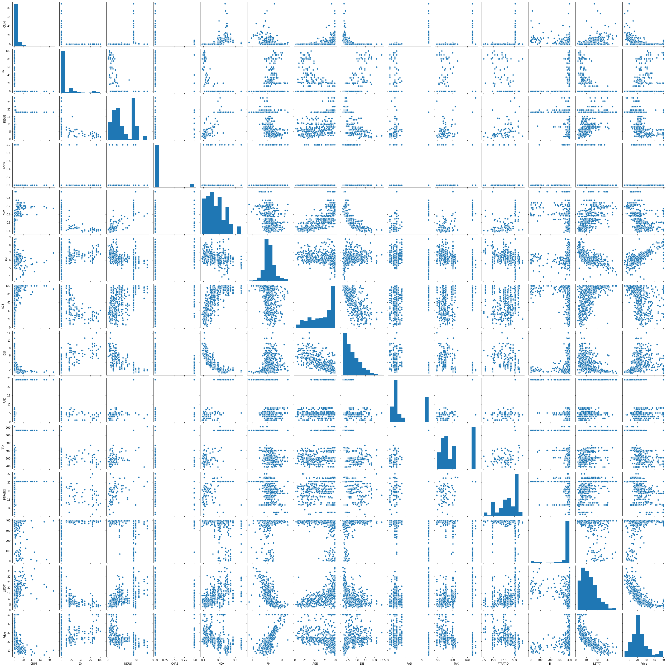
Data Visualization
sns.pairplot(data)
<seaborn.axisgrid.PairGrid at 0x7f1e07874f60>
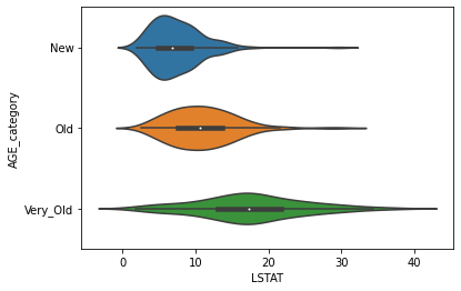
CREARE VARIABILI CATEGORICHE PER VARIABILI CONTINUE E VISUALIZZARLE
df_cat=data.copy()
def get_age_category(x):
    if x < 50:
        return 'New'
    elif 50 <= x < 85:
        return 'Old'
    else:
        return 'Very_Old'

df_cat['AGE_category'] = df_cat.AGE.apply(get_age_category)
df_cat.groupby('AGE_category').size()
AGE_category
New         147
Old         149
Very_Old    210
dtype: int64
sns.violinplot(x='LSTAT', y='AGE_category', data=df_cat, order=['New', 'Old','Very_Old']);
sns.pairplot(df_cat, hue='AGE_category',hue_order=['New', 'Old','Very_Old']);
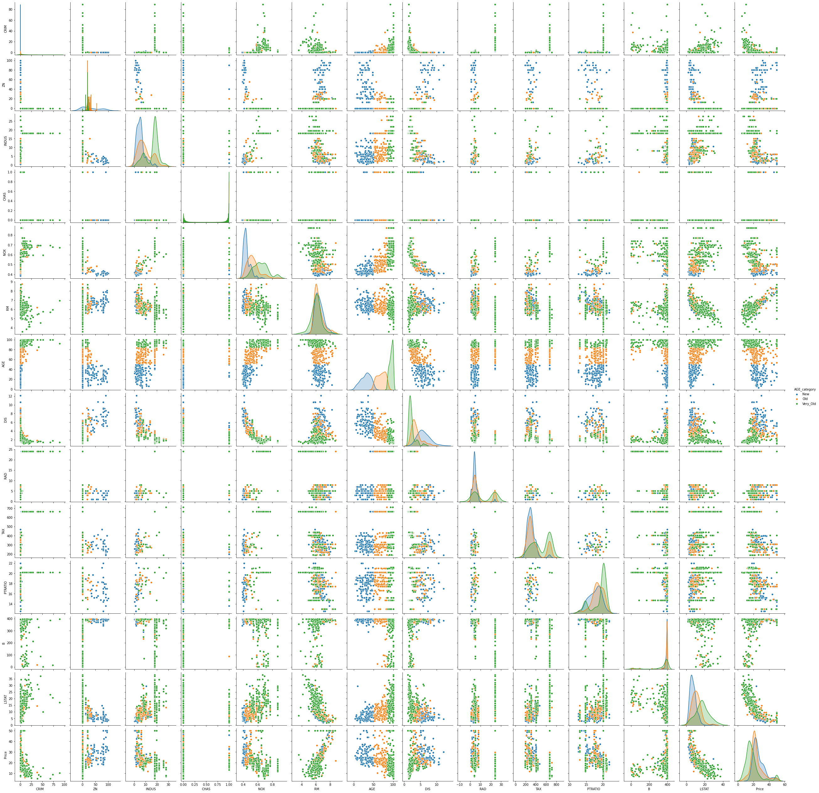
############ fine esperimento
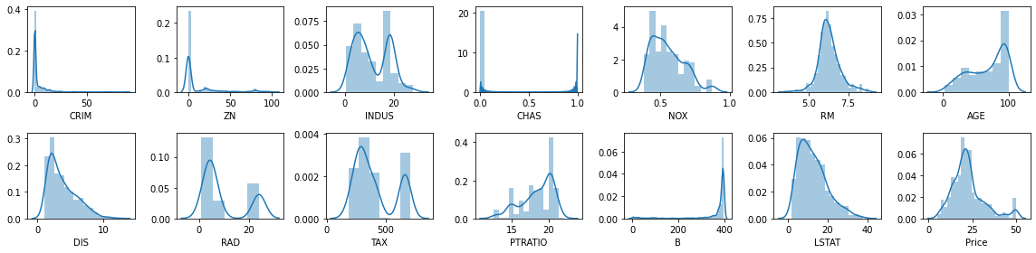
rows = 2
cols = 7

fig, ax = plt.subplots(nrows= rows, ncols= cols, figsize = (16,4))

col = data.columns
index = 0

for i in range(rows):
    for j in range(cols):
        sns.distplot(data[col[index]], ax = ax[i][j])
        index = index + 1

plt.tight_layout()
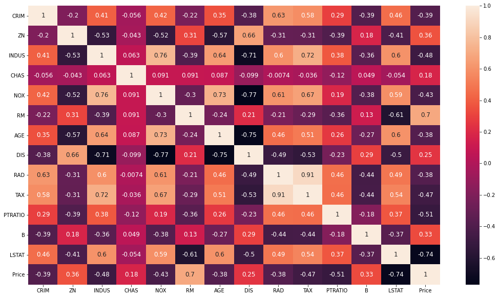
corrmat = data.corr()
corrmat
| CRIM | ZN | INDUS | CHAS | NOX | RM | AGE | DIS | RAD | TAX | PTRATIO | B | LSTAT | Price | |
|---|---|---|---|---|---|---|---|---|---|---|---|---|---|---|
| CRIM | 1.000000 | -0.200469 | 0.406583 | -0.055892 | 0.420972 | -0.219247 | 0.352734 | -0.379670 | 0.625505 | 0.582764 | 0.289946 | -0.385064 | 0.455621 | -0.388305 |
| ZN | -0.200469 | 1.000000 | -0.533828 | -0.042697 | -0.516604 | 0.311991 | -0.569537 | 0.664408 | -0.311948 | -0.314563 | -0.391679 | 0.175520 | -0.412995 | 0.360445 |
| INDUS | 0.406583 | -0.533828 | 1.000000 | 0.062938 | 0.763651 | -0.391676 | 0.644779 | -0.708027 | 0.595129 | 0.720760 | 0.383248 | -0.356977 | 0.603800 | -0.483725 |
| CHAS | -0.055892 | -0.042697 | 0.062938 | 1.000000 | 0.091203 | 0.091251 | 0.086518 | -0.099176 | -0.007368 | -0.035587 | -0.121515 | 0.048788 | -0.053929 | 0.175260 |
| NOX | 0.420972 | -0.516604 | 0.763651 | 0.091203 | 1.000000 | -0.302188 | 0.731470 | -0.769230 | 0.611441 | 0.668023 | 0.188933 | -0.380051 | 0.590879 | -0.427321 |
| RM | -0.219247 | 0.311991 | -0.391676 | 0.091251 | -0.302188 | 1.000000 | -0.240265 | 0.205246 | -0.209847 | -0.292048 | -0.355501 | 0.128069 | -0.613808 | 0.695360 |
| AGE | 0.352734 | -0.569537 | 0.644779 | 0.086518 | 0.731470 | -0.240265 | 1.000000 | -0.747881 | 0.456022 | 0.506456 | 0.261515 | -0.273534 | 0.602339 | -0.376955 |
| DIS | -0.379670 | 0.664408 | -0.708027 | -0.099176 | -0.769230 | 0.205246 | -0.747881 | 1.000000 | -0.494588 | -0.534432 | -0.232471 | 0.291512 | -0.496996 | 0.249929 |
| RAD | 0.625505 | -0.311948 | 0.595129 | -0.007368 | 0.611441 | -0.209847 | 0.456022 | -0.494588 | 1.000000 | 0.910228 | 0.464741 | -0.444413 | 0.488676 | -0.381626 |
| TAX | 0.582764 | -0.314563 | 0.720760 | -0.035587 | 0.668023 | -0.292048 | 0.506456 | -0.534432 | 0.910228 | 1.000000 | 0.460853 | -0.441808 | 0.543993 | -0.468536 |
| PTRATIO | 0.289946 | -0.391679 | 0.383248 | -0.121515 | 0.188933 | -0.355501 | 0.261515 | -0.232471 | 0.464741 | 0.460853 | 1.000000 | -0.177383 | 0.374044 | -0.507787 |
| B | -0.385064 | 0.175520 | -0.356977 | 0.048788 | -0.380051 | 0.128069 | -0.273534 | 0.291512 | -0.444413 | -0.441808 | -0.177383 | 1.000000 | -0.366087 | 0.333461 |
| LSTAT | 0.455621 | -0.412995 | 0.603800 | -0.053929 | 0.590879 | -0.613808 | 0.602339 | -0.496996 | 0.488676 | 0.543993 | 0.374044 | -0.366087 | 1.000000 | -0.737663 |
| Price | -0.388305 | 0.360445 | -0.483725 | 0.175260 | -0.427321 | 0.695360 | -0.376955 | 0.249929 | -0.381626 | -0.468536 | -0.507787 | 0.333461 | -0.737663 | 1.000000 |
plt.subplots(figsize = (18, 10))
sns.heatmap(corrmat, annot = True, annot_kws={'size': 12});
corrmat.index.values
array(['CRIM', 'ZN', 'INDUS', 'CHAS', 'NOX', 'RM', 'AGE', 'DIS', 'RAD',
       'TAX', 'PTRATIO', 'B', 'LSTAT', 'Price'], dtype=object)
##1
def getCorrelatedFeature(corrdata, threshold):
    feature = []
    value = []

    for i, index in enumerate(corrdata.index):
        if abs(corrdata[index])> threshold:
            feature.append(index)
            value.append(corrdata[index])

    df = pd.DataFrame(data = value, index = feature, columns=['Corr Value'])
    return df
# Prendi la colonna Price del dataframe data, applica la treshold e includi in questo dataframe le features
threshold = 0.50
corr_value = getCorrelatedFeature(corrmat['Price'], threshold)
corr_value
| Corr Value | |
|---|---|
| RM | 0.695360 |
| PTRATIO | -0.507787 |
| LSTAT | -0.737663 |
| Price | 1.000000 |
corr_value.index.values
array(['RM', 'PTRATIO', 'LSTAT', 'Price'], dtype=object)
correlated_data = data[corr_value.index]
correlated_data.head()
| RM | PTRATIO | LSTAT | Price | |
|---|---|---|---|---|
| 0 | 6.575 | 15.3 | 4.98 | 24.0 |
| 1 | 6.421 | 17.8 | 9.14 | 21.6 |
| 2 | 7.185 | 17.8 | 4.03 | 34.7 |
| 3 | 6.998 | 18.7 | 2.94 | 33.4 |
| 4 | 7.147 | 18.7 | 5.33 | 36.2 |
correlated_data.shape
(506, 4)
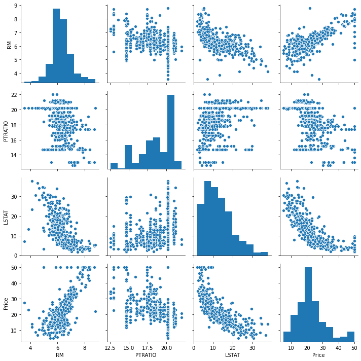
sns.pairplot(correlated_data)
plt.tight_layout()
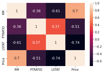
sns.heatmap(correlated_data.corr(), annot=True, annot_kws={'size': 12});
Shuffle and Split Data
X = correlated_data.drop(labels=['Price'], axis = 1)
y = correlated_data['Price']
X.head()
| RM | PTRATIO | LSTAT | |
|---|---|---|---|
| 0 | 6.575 | 15.3 | 4.98 |
| 1 | 6.421 | 17.8 | 9.14 |
| 2 | 7.185 | 17.8 | 4.03 |
| 3 | 6.998 | 18.7 | 2.94 |
| 4 | 7.147 | 18.7 | 5.33 |
X_train, X_test, y_train, y_test = train_test_split(X, y, test_size = 0.2, random_state = 0)
X_train.shape, X_test.shape
((404, 3), (102, 3))
Start train the model
model = LinearRegression()
model.fit(X_train, y_train)
LinearRegression(copy_X=True, fit_intercept=True, n_jobs=None, normalize=False)
y_predict = model.predict(X_test)
df = pd.DataFrame(data = [y_predict, y_test])
df = df.T
df.columns = ['predetti', 'reali_test']
df
| predetti | reali_test | |
|---|---|---|
| 0 | 27.609031 | 22.6 |
| 1 | 22.099034 | 50.0 |
| 2 | 26.529255 | 23.0 |
| 3 | 12.507986 | 8.3 |
| 4 | 22.254879 | 21.2 |
| ... | ... | ... |
| 97 | 28.271228 | 24.7 |
| 98 | 18.467419 | 14.1 |
| 99 | 18.558070 | 18.7 |
| 100 | 24.681964 | 28.1 |
| 101 | 20.826879 | 19.8 |
102 rows × 2 columns
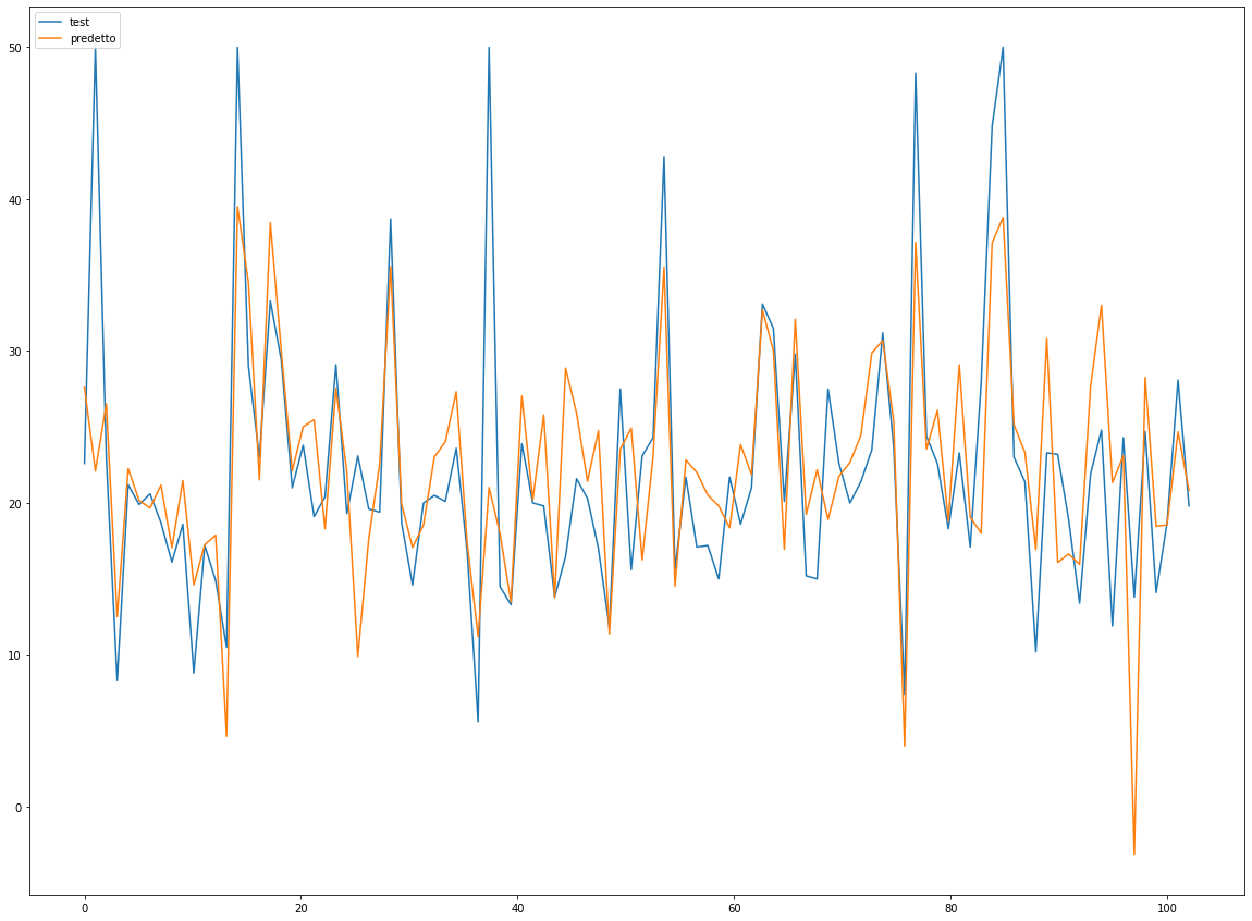
length = y_predict.shape[0] #
x = np.linspace(0,length,length)


plt.figure(figsize=(20,15))
plt.plot(x, y_test, label='test')
plt.plot(x, y_predict, label='predetto')
plt.legend(loc=2);
Defining performance metrics
It is difficult to measure the quality of a given model without quantifying its performance over training and testing. This is typically done using some type of performance metric, whether it is through calculating some type of error, the goodness of fit, or some other useful measurement. For this project, you will be calculating the coefficient of determination, R2, to quantify your model’s performance. The coefficient of determination for a model is a useful statistic in regression analysis, as it often describes how “good” that model is at making predictions.
The values for R2 range from 0 to 1, which captures the percentage of squared correlation between the predicted and actual values of the target variable. A model with an R2 of 0 always fails to predict the target variable, whereas a model with an R2 of 1 perfectly predicts the target variable. Any value between 0 and 1 indicates what percentage of the target variable, using this model, can be explained by the features. A model can be given a negative R2 as well, which indicates that the model is no better than one that naively predicts the mean of the target variable.
For the performance_metric function in the code cell below, you will need to implement the following:
Use r2_score from sklearn.metrics to perform a performance calculation between y_true and y_predict. Assign the performance score to the score variable.
Regression Evaluation Metrics
Here are three common evaluation metrics for regression problems:
Mean Absolute Error (MAE) is the mean of the absolute value of the errors:
Mean Squared Error (MSE) is the mean of the squared errors:
Root Mean Squared Error (RMSE) is the square root of the mean of the squared errors:
Comparing these metrics:
MAE is the easiest to understand, because it’s the average error. MSE is more popular than MAE, because MSE “punishes” larger errors, which tends to be useful in the real world. RMSE is even more popular than MSE, because RMSE is interpretable in the “y” units. All of these are loss functions, because we want to minimize them.
from sklearn.metrics import r2_score
correlated_data.columns
Index(['RM', 'PTRATIO', 'LSTAT', 'Price'], dtype='object')
score = r2_score(y_test, y_predict)
mae = mean_absolute_error(y_test, y_predict)
mse = mean_squared_error(y_test, y_predict)

print('r2_score: ', score)
print('mae: ', mae)
print('mse: ', mse)
r2_score:  0.48816420156925067
mae:  4.404434993909257
mse:  41.67799012221683
##2

total_features = []
total_features_name = []
selected_correlation_value = []
r2_scores = []
mae_value = []
mse_value = []

def performance_metrics(features, th, y_true, y_pred):
    score = r2_score(y_true, y_pred)
    mae = mean_absolute_error(y_true, y_pred)
    mse = mean_squared_error(y_true, y_pred)

    total_features.append(len(features)-1)
    total_features_name.append(str(features))
    selected_correlation_value.append(th)
    r2_scores.append(score)
    mae_value.append(mae)
    mse_value.append(mse)

    metrics_dataframe = pd.DataFrame(data= [total_features_name, total_features, selected_correlation_value, r2_scores, mae_value, mse_value],
                                    index = ['features name', '#feature', 'corr_value', 'r2_score', 'MAE', 'MSE'])
    return metrics_dataframe.T
performance_metrics(correlated_data.columns.values, threshold, y_test, y_predict)
| features name | #feature | corr_value | r2_score | MAE | MSE | |
|---|---|---|---|---|---|---|
| 0 | ['RM' 'PTRATIO' 'LSTAT' 'Price'] | 3 | 0.5 | 0.488164 | 4.40443 | 41.678 |
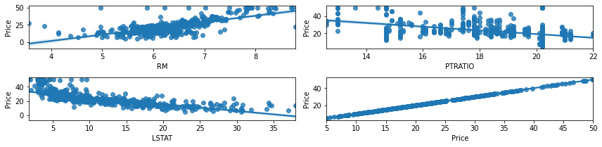
regression plot of the features correlated with the price
rows = 2
cols = 2
fig, ax = plt.subplots(nrows=rows, ncols=cols, figsize = (12, 3))

col = correlated_data.columns
index = 0

for i in range(rows):
    for j in range(cols):
        sns.regplot(x = correlated_data[col[index]], y = correlated_data['Price'], ax = ax[i][j])
        index = index + 1
fig.tight_layout()
Let’s find out other combination of columns to get better accuracy >60%
corrmat['Price']
CRIM      -0.388305
ZN         0.360445
INDUS     -0.483725
CHAS       0.175260
NOX       -0.427321
RM         0.695360
AGE       -0.376955
DIS        0.249929
RAD       -0.381626
TAX       -0.468536
PTRATIO   -0.507787
B          0.333461
LSTAT     -0.737663
Price      1.000000
Name: Price, dtype: float64
threshold = 0.60
corr_value = getCorrelatedFeature(corrmat['Price'], threshold)
corr_value
| Corr Value | |
|---|---|
| RM | 0.695360 |
| LSTAT | -0.737663 |
| Price | 1.000000 |
correlated_data = data[corr_value.index]
correlated_data.head()
| RM | LSTAT | Price | |
|---|---|---|---|
| 0 | 6.575 | 4.98 | 24.0 |
| 1 | 6.421 | 9.14 | 21.6 |
| 2 | 7.185 | 4.03 | 34.7 |
| 3 | 6.998 | 2.94 | 33.4 |
| 4 | 7.147 | 5.33 | 36.2 |
##3

def get_y_predict(corr_data):
    X = corr_data.drop(labels = ['Price'], axis = 1)
    y = corr_data['Price']

    X_train, X_test, y_train, y_test = train_test_split(X, y, test_size = 0.2, random_state = 0)
    model = LinearRegression()
    model.fit(X_train, y_train)
    y_predict = model.predict(X_test)
    return y_predict
y_predict = get_y_predict(correlated_data)
performance_metrics(correlated_data.columns.values, threshold, y_test, y_predict)
| features name | #feature | corr_value | r2_score | MAE | MSE | |
|---|---|---|---|---|---|---|
| 0 | ['RM' 'PTRATIO' 'LSTAT' 'Price'] | 3 | 0.5 | 0.488164 | 4.40443 | 41.678 |
| 1 | ['RM' 'LSTAT' 'Price'] | 2 | 0.6 | 0.540908 | 4.14244 | 37.3831 |
Let’s find out other combination of columns to get better accuracy >70%
corrmat['Price']
CRIM      -0.388305
ZN         0.360445
INDUS     -0.483725
CHAS       0.175260
NOX       -0.427321
RM         0.695360
AGE       -0.376955
DIS        0.249929
RAD       -0.381626
TAX       -0.468536
PTRATIO   -0.507787
B          0.333461
LSTAT     -0.737663
Price      1.000000
Name: Price, dtype: float64
threshold = 0.70
corr_value = getCorrelatedFeature(corrmat['Price'], threshold)
corr_value
| Corr Value | |
|---|---|
| LSTAT | -0.737663 |
| Price | 1.000000 |
correlated_data = data[corr_value.index]
correlated_data.head()
| LSTAT | Price | |
|---|---|---|
| 0 | 4.98 | 24.0 |
| 1 | 9.14 | 21.6 |
| 2 | 4.03 | 34.7 |
| 3 | 2.94 | 33.4 |
| 4 | 5.33 | 36.2 |
y_predict = get_y_predict(correlated_data)
performance_metrics(correlated_data.columns.values, threshold, y_test, y_predict)
| features name | #feature | corr_value | r2_score | MAE | MSE | |
|---|---|---|---|---|---|---|
| 0 | ['RM' 'PTRATIO' 'LSTAT' 'Price'] | 3 | 0.5 | 0.488164 | 4.40443 | 41.678 |
| 1 | ['RM' 'LSTAT' 'Price'] | 2 | 0.6 | 0.540908 | 4.14244 | 37.3831 |
| 2 | ['LSTAT' 'Price'] | 1 | 0.7 | 0.430957 | 4.86401 | 46.3363 |
Normalization and Standardization
Standardization = Gaussian with zero mean and unit variance.
Z is rescaled such that any specific z will now be 0 ≤ z ≤ 1, and is done through this formula:
model = LinearRegression(normalize=True)
model.fit(X_train, y_train)
LinearRegression(copy_X=True, fit_intercept=True, n_jobs=None, normalize=True)
y_predict = model.predict(X_test)
r2_score(y_test, y_predict)
0.4881642015692508
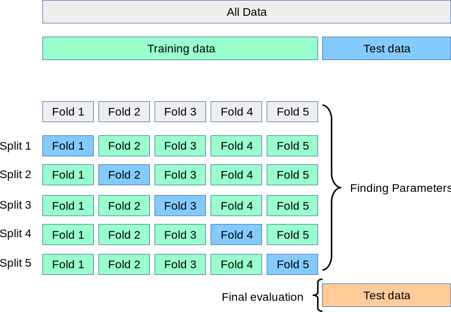
Cross Validation
from IPython.display import Image
Image(url='https://frenzy86.s3.eu-west-2.amazonaws.com/fav/cross_val.png',width=600,height=300)
import numpy as np
from sklearn.model_selection import train_test_split
from sklearn import datasets
from sklearn.linear_model import LinearRegression
boston = datasets.load_boston()
boston.data.shape, boston.target.shape
((506, 13), (506,))
X_train, X_test, y_train, y_test = train_test_split(
    boston.data, boston.target, test_size=0.3, random_state=0)
X_train.shape, y_train.shape
X_test.shape, y_test.shape

model = LinearRegression()

model.fit(X_train, y_train)
model.score(X_test, y_test) #R^2
0.6733825506400171
from sklearn.model_selection import cross_val_score

scores = cross_val_score(model, boston.data, boston.target, cv=5)
scores
array([ 0.63919994, 0.71386698, 0.58702344, 0.07923081, -0.25294154])