.ipynb .pdf

On this page

Decision Tree

Important Considerations

PROS	CONS
Easy to visualize and Interpret	Prone to overfitting
No normalization of Data Necessary	Ensemble needed for better performance
Handles mixed feature types

Iris Example

Use measurements to predict species

Iris Example Use measurements to predict species

%matplotlib inline
import matplotlib.pyplot as plt
from sklearn.datasets import load_iris
from sklearn import tree
from sklearn.datasets import load_iris
from sklearn.tree import DecisionTreeClassifier
from sklearn.model_selection import train_test_split

import seaborn as sns
iris = sns.load_dataset('iris')
iris.head()

	sepal_length	sepal_width	petal_length	petal_width	species
0	5.1	3.5	1.4	0.2	setosa
1	4.9	3.0	1.4	0.2	setosa
2	4.7	3.2	1.3	0.2	setosa
3	4.6	3.1	1.5	0.2	setosa
4	5.0	3.6	1.4	0.2	setosa

#split the data
iris = load_iris()
X_train, X_test, y_train, y_test = train_test_split(iris.data, iris.target)

len(X_test)

38

#load classifier
classifier = tree.DecisionTreeClassifier()

#fit train data
classifier = classifier.fit(X_train, y_train)

#examine score
classifier.score(X_train, y_train)

1.0

#against test set
classifier.score(X_test, y_test)

0.9210526315789473

How would specific flower be classified?

If we have a flower that has:

• Sepal.Length = 1.0

• Sepal.Width = 0.3

• Petal.Length = 1.4

• Petal.Width = 2.1

classifier.predict_proba([[1.0, 0.3, 1.4, 2.1]])

array([[0., 0., 1.]])

#cross validation
from sklearn.model_selection import cross_val_score
cross_val_score(classifier, X_train, y_train, cv=10)

array([0.83333333, 0.91666667, 0.90909091, 1.        , 0.90909091,
       0.90909091, 1.        , 1.        , 0.72727273, 1.        ])

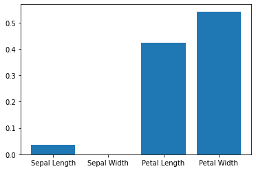
How important are different features?

1. List item

2. List item

#list of feature importance
classifier.feature_importances_

array([0.03579418, 0.        , 0.42226156, 0.54194426])

importance = classifier.feature_importances_

plt.bar(['Sepal Length', 'Sepal Width', 'Petal Length', 'Petal Width'], importance)

<BarContainer object of 4 artists>

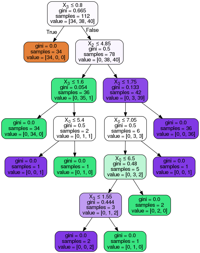
Visualizing Decision Tree

%%capture
!pip install --upgrade scikit-learn==0.20.3 pydotplus

from sklearn.externals.six import StringIO  
from IPython.display import Image  
from sklearn.tree import export_graphviz
import pydotplus

dot_data = StringIO()
export_graphviz(classifier, out_file=dot_data,  filled=True, rounded=True, special_characters=True)
graph = pydotplus.graph_from_dot_data(dot_data.getvalue())  
Image(graph.create_png())

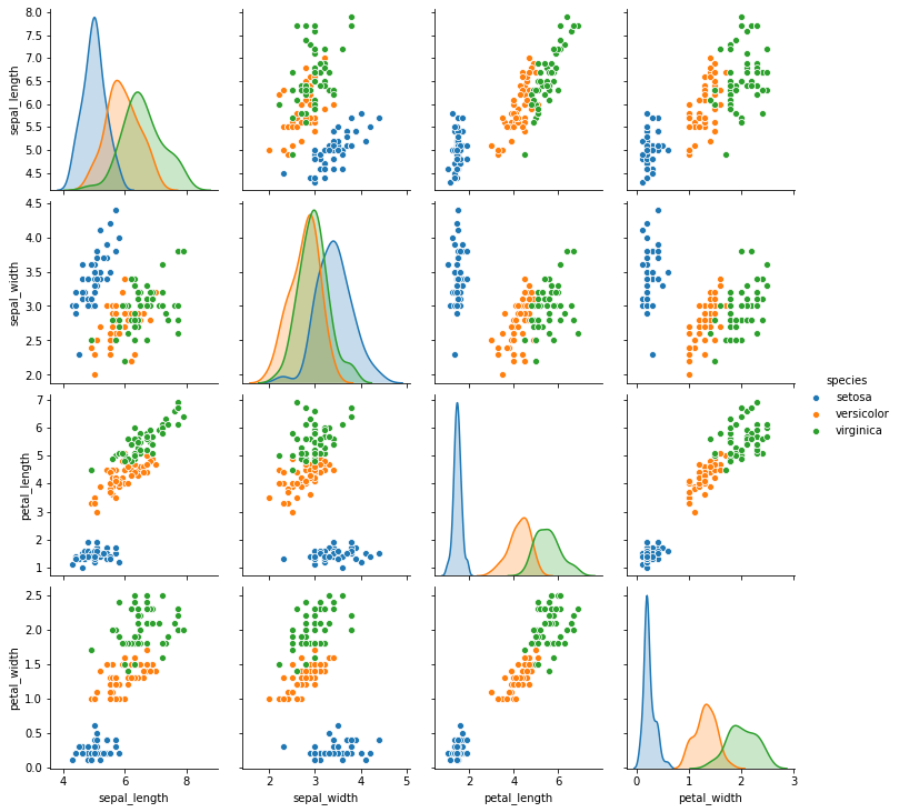
What’s Happening with Decision Tree

import seaborn as sns
iris = sns.load_dataset('iris')
sns.pairplot(data = iris, hue = 'species');

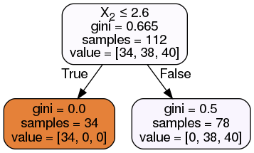
Pre-pruning: Avoiding Over-fitting

• max_depth: limits depth of tree

• max_leaf_nodes: limits how many leafs

• min_samples_leaf: limits splits to happen when only certain number of samples exist

classifier = DecisionTreeClassifier(max_depth = 1).fit(X_train, y_train)

classifier.score(X_train, y_train)

0.6607142857142857

classifier.score(X_test, y_test)

0.6842105263157895

dot_data = StringIO()
export_graphviz(classifier, out_file=dot_data,  filled=True, rounded=True, special_characters=True)
graph = pydotplus.graph_from_dot_data(dot_data.getvalue())  
Image(graph.create_png())

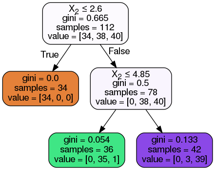
classifier = DecisionTreeClassifier(max_depth = 2).fit(X_train, y_train)

classifier.score(X_train, y_train)

0.9642857142857143

classifier.score(X_test, y_test)

0.9210526315789473

dot_data = StringIO()
export_graphviz(classifier, out_file=dot_data,  filled=True, rounded=True, special_characters=True)
graph = pydotplus.graph_from_dot_data(dot_data.getvalue())  
Image(graph.create_png())

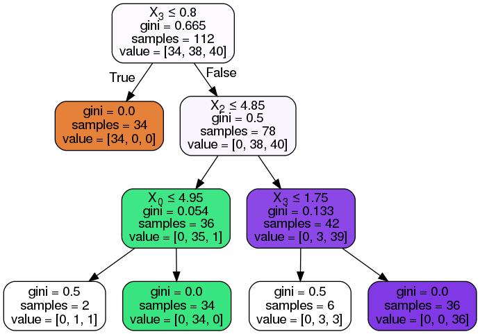
classifier = DecisionTreeClassifier(max_depth = 3).fit(X_train, y_train)
classifier.score(X_train, y_train)

0.9642857142857143

classifier.score(X_test, y_test)

0.9210526315789473

Confusion Matrix

from sklearn.metrics import classification_report
import sklearn.metrics
from sklearn.metrics import confusion_matrix

classifier=classifier.fit(X_train,y_train)

predictions=classifier.predict(X_test)

mat = confusion_matrix(y_test, predictions)
sns.heatmap(mat.T, square=True, annot=True, fmt='d', cbar=False)
plt.xlabel('true label')
plt.ylabel('predicted label');

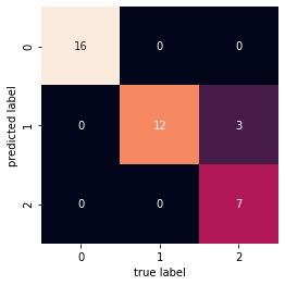
sklearn.metrics.confusion_matrix(y_test, predictions)

array([[16,  0,  0],
       [ 0, 12,  0],
       [ 0,  3,  7]])

dot_data2 = StringIO()
export_graphviz(classifier, out_file=dot_data2,  
                filled=True, rounded=True,
                special_characters=True)
graph2 = pydotplus.graph_from_dot_data(dot_data2.getvalue())  
Image(graph2.create_png())

sklearn.metrics.accuracy_score(y_test, predictions)

0.9210526315789473

Binary classifier 5 or not 5 ? Clustering